if confidence level increases what happens to width

Allow's say yous have a sample mean, y'all may wish to know what confidence intervals you tin place on that mean. Colloquially: "I want an interval that I tin be P% sure contains the truthful mean". (On a technical point, note that the interval either contains the true mean or it does non: the meaning of the confidence level is subtly unlike from this colloquialism. More background information tin can exist plant on the NIST site).

The formula for the interval can be expressed as:

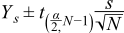
Where, Y_{due south} is the sample mean, due south is the sample standard deviation, N is the sample size, [blastoff] is the desired significance level and t_{(α/ii,North-ane)} is the upper critical value of the Students-t distribution with N-1 degrees of liberty.

Note

The quantity α is the maximum acceptable chance of falsely rejecting the goose egg-hypothesis. The smaller the value of α the greater the strength of the examination. The confidence level of the examination is defined equally i - α, and often expressed as a percentage. And then for case a significance level of 0.05, is equivalent to a 95% conviction level. Refer to "What are confidence intervals?" in NIST/SEMATECH eastward-Handbook of Statistical Methods. for more information.

From the formula, it should be clear that:

• The width of the conviction interval decreases as the sample size increases.
• The width increases as the standard deviation increases.
• The width increases as the confidence level increases (0.5 towards 0.99999 - stronger).
• The width increases as the significance level decreases (0.5 towards 0.00000...01 - stronger).

The following instance code is taken from the example plan students_t_single_sample.cpp.

We'll brainstorm by defining a process to calculate intervals for various conviction levels; the procedure volition print these out every bit a table:

          #include          <          boost          /          math          /          distributions          /          students_t          .          hpp          >          #include          <          iostream          >          #include          <          iomanip          >          using          namespace          boost          ::          math          ;          using          namespace          std          ;          void          confidence_limits_on_mean          (          double          Sm          ,                    double          Sd          ,                    unsigned          Sn          )          {          using          namespace          std          ;          using          namespace          heave          ::          math          ;                    cout          <<          "__________________________________\n"          "2-Sided Confidence Limits For Hateful\due north"          "__________________________________\north\n"          ;          cout          <<          setprecision          (          seven          );          cout          <<          setw          (          40          )          <<          left          <<          "Number of Observations"          <<          "=  "          <<          Sn          <<          "\north"          ;          cout          <<          setw          (          twoscore          )          <<          left          <<          "Mean"          <<          "=  "          <<          Sm          <<          "\n"          ;          cout          <<          setw          (          40          )          <<          left          <<          "Standard Difference"          <<          "=  "          <<          Sd          <<          "\n"          ;        

We'll define a table of significance/risk levels for which we'll compute intervals:

          double          alpha          []          =          {          0.five          ,          0.25          ,          0.1          ,          0.05          ,          0.01          ,          0.001          ,          0.0001          ,          0.00001          };        

Note that these are the complements of the confidence/probability levels: 0.5, 0.75, 0.9 .. 0.99999).

Adjacent nosotros'll declare the distribution object we'll demand, annotation that the degrees of freedom parameter is the sample size less one:

          students_t          dist          (          Sn          -          1          );        

Near of what follows in the program is pretty printing, so let's focus on the calculation of the interval. First nosotros need the t-statistic, computed using the quantile office and our significance level. Note that since the significance levels are the complement of the probability, we take to wrap the arguments in a call to complement(...) :

          double          T          =          quantile          (          complement          (          dist          ,          alpha          [          i          ]          /          2          ));        

Note that alpha was divided by two, since nosotros'll be calculating both the upper and lower bounds: had we been interested in a single sided interval then we would take omitted this step.

Now to complete the picture, nosotros'll get the (one-sided) width of the interval from the t-statistic past multiplying by the standard deviation, and dividing by the square root of the sample size:

          double          w          =          T          *          Sd          /          sqrt          (          double          (          Sn          ));        

The 2-sided interval is and so the sample mean plus and minus this width.

And apart from some more pretty-printing that completes the procedure.

Let's take a look at some sample output, showtime using the Estrus flow information from the NIST site. The information set was collected past Bob Zarr of NIST in January, 1990 from a heat catamenia meter scale and stability analysis. The respective dataplot output for this test can be found in department three.5.ii of the NIST/SEMATECH e-Handbook of Statistical Methods..

          __________________________________    2-Sided Conviction Limits For Hateful    __________________________________     Number of Observations                  =  195    Mean                                    =  9.26146    Standard Deviation                      =  0.02278881      ___________________________________________________________________    Confidence       T           Interval          Lower          Upper     Value (%)     Value          Width            Limit          Limit    ___________________________________________________________________        l.000     0.676       1.103e-003        9.26036        9.26256        75.000     ane.154       1.883e-003        9.25958        9.26334        90.000     1.653       two.697e-003        9.25876        9.26416        95.000     1.972       3.219e-003        9.25824        9.26468        99.000     ii.601       4.245e-003        9.25721        ix.26571        99.900     iii.341       5.453e-003        9.25601        9.26691        99.990     3.973       6.484e-003        nine.25498        9.26794        99.999     4.537       7.404e-003        ix.25406        9.26886        

As you tin can see the big sample size (195) and small standard deviation (0.023) accept combined to give very small intervals, indeed we tin can be very confident that the truthful mean is 9.2.

For comparing the next case data output is taken from P.Thou.Hou, O. W. Lau & G.C. Wong, Analyst (1983) vol. 108, p 64. and from Statistics for Analytical Chemical science, 3rd ed. (1994), pp 54-55 J. C. Miller and J. N. Miller, Ellis Horwood ISBN 0 13 0309907. The values result from the determination of mercury by cold-vapour atomic absorption.

          __________________________________    ii-Sided Confidence Limits For Hateful    __________________________________     Number of Observations                  =  iii    Hateful                                    =  37.8000000    Standard Deviation                      =  0.9643650      ___________________________________________________________________    Confidence       T           Interval          Lower          Upper     Value (%)     Value          Width            Limit          Limit    ___________________________________________________________________        l.000     0.816            0.455       37.34539       38.25461        75.000     1.604            0.893       36.90717       38.69283        90.000     two.920            1.626       36.17422       39.42578        95.000     iv.303            2.396       35.40438       forty.19562        99.000     9.925            five.526       32.27408       43.32592        99.900    31.599           17.594       20.20639       55.39361        99.990    99.992           55.673      -17.87346       93.47346        99.999   316.225          176.067     -138.26683      213.86683        

This time the fact that there are but iii measurements leads to much wider intervals, indeed such big intervals that it's difficult to exist very confident in the location of the hateful.

murdockpowle1955.blogspot.com

Source: https://www.boost.org/doc/libs/1_41_0/libs/math/doc/sf_and_dist/html/math_toolkit/dist/stat_tut/weg/st_eg/tut_mean_intervals.html

Share this post